Population protocols
The population protocol model (PP, for short) is an abstract computational model for distributed algorithms. A step of computation, in this model, corresponds to the modification of the states of two neighbor nodes in an atomic way. Furthermore, in order to break local symmetry during the interaction, both nodes play different roles: one is initiator, the other is responder.
An execution typically involves a scheduler and an algorithm. The scheduler (also called adversary or daemon) is responsible for chosing which pair of nodes will interact in the current round, while the algorithm determines what effect such interaction will have. The algorithm also determines what the initial states are (with possibly a distinguished state for some particular nodes).
Structure of a protocol
Before writing the scheduler, let us define a class PPNode that encapsulates the features of any population protocol, and of which our own protocols will inherit. These features are materialized as three abstract methods that our protocols (derived class) must implement (possibly in an empty way). They correspond to the same elements as above, made more explicit:
- What the default initial state is? The corresponding assignments are to be made in the
onStart()method, which is (conveniently) called by JBotSim on a node that joins the topology (thus on all nodes). - What the distinguished initial state is, if applicable (e.g. a leader node)? The corresponding assignments are to be made in the
onSelection()method, which is called when a node is selected by the user (middle click on PCs, command-shift click on macs). - What changes an interaction between two nodes make on those nodes states (i.e. the main operations of the algorithm)? The corresponding code is to be added in the
interactWith()method.
Here is the corresponding abstract class (PPNode).
import io.jbotsim.core.Node;

public abstract class PPNode extends Node {
    // Assign default initial state to underlying node
    public abstract void onStart();
    // Assign distinguished initial state to underlying node
    public abstract void onSelection();
    // Execute interaction (from the initiator side)
    public abstract void interactWith(Node responder);
}
Example: basic protocol for information dissemination
In this protocol, a piece of information is initially located at some (distinguished) node, while others are uninformed. An interaction then consists in testing if one of the two nodes is informed while the other is not, and if so, the other becomes informed. We might represent this rule graphically as follows: o--x → o--o. For the sake of visualization, we encode the states as colors, with informed nodes in red and uninformed nodes in blue. Thus initially, all nodes will be in blue, except one selected by the user (thus executing the onSelection() method and turning red). Here is the corresponding code.
import io.jbotsim.core.Color;
import io.jbotsim.core.Node;

public class PPNodeAlgo1 extends PPNode {
    @Override
    public void onStart() {
        setColor(Color.blue);
    }
    @Override
    public void onSelection() {
        setColor(Color.red);
    }
    @Override
    public void interactWith(Node responder) {
        if (this.getColor() == Color.red && responder.getColor() == Color.blue)
            responder.setColor(Color.red);
        else if (this.getColor() == Color.blue && responder.getColor() == Color.red)
            this.setColor(Color.red);
    }
}
Here is what this protocol will produce (after you've added the scheduler and main methods explained further below). A video is also available here.
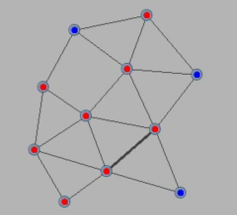
Execution of a population protocol.
The scheduler
Let's now write a (global) scheduler that decides in each round which pair of nodes interact. Here, the choice is made at random (u.a.r.) among all the network links and interaction is triggered on the corresponding nodes, through a call to method interactWith on the initiator node. Here is the code.
import io.jbotsim.core.Link;
import io.jbotsim.core.Topology;
import io.jbotsim.core.event.ClockListener;

import java.util.List;

public class PPScheduler implements ClockListener {
    Topology tp;

    public PPScheduler(Topology topology) {
        tp = topology;
        tp.addClockListener(this);
    }

    @Override
    public void onClock() {
        // Retrieve all links
        List<Link> links = tp.getLinks();
        if ( ! links.isEmpty() ) {
            // Pick a link at random
            Link selectedLink = links.get((int) (Math.random() * links.size()));
            // Make it bold for visualization
            drawInteraction(selectedLink);
            // Pick initiator side at random
            PPNode initiator = (PPNode) selectedLink.endpoint((int) (Math.random() * 2));
            PPNode responder = (PPNode) selectedLink.getOtherEndpoint(initiator);
            // Perform interaction
            initiator.interactWith(responder);
        }
    }

    // Draw a given link in bold (and unbold others)
    public void drawInteraction(Link selectedLink){
        for (Link link : tp.getLinks())
            link.setWidth(1);
        selectedLink.setWidth(3);
    }
}
main method (and class)
We are almost there. What remains is only to do the settings in a main() method, namely, create a topology; specify what type of node must be used by default (PPNodeAlgo1); slow down execution for visualization to 100ms a round; and finally create both the scheduler and the viewer.
import io.jbotsim.core.Topology;
import io.jbotsim.ui.JViewer;

public class MainPP {
    public static void main(String[] args) {
        Topology tp = new Topology();
        tp.setDefaultNodeModel(PPNodeAlgo1.class);
        tp.setTimeUnit(100);
        new PPScheduler(tp);
        new JViewer(tp);
        tp.start();
    }
}
Training
Q1. Check that everything works as expected. Recall that you can select the initial informed node through middle click (on PCs), or command-shift click (on macs).
In the following, we will consider three protocols whose goal is to count how many nodes there are in the network. These protocols will go from the most basic (and very limited) to the better.
Counting v1: In this protocol, one distinguished node (called the counter) counts all the nodes that it interacts with. Initially, all the other nodes are in the uncounted state, then some of them become counted as the execution progresses. The distinction between counted and uncounted is important to prevent multiple counting of a same node.
Q2. Implement this counting protocol into a dedicated node class extending PPNode. You may represent the main states (i.e. counter, counted, and uncounted) by three colors, and the count by an integer variable that only the counter will effectively use.
→ Visualization tip: you can override the toString() method to return the current count when called on the counter node (and an empty string otherwise). This will show in the tooltip of that node when you pass the mouse over it.
Q3. The previous protocol is very limited. What basic condition must the graph satisfy to give a chance of success to the counter (i.e. to converge eventually to the total number of nodes)? In the early time of population protocols, a classical assumption was that all pairs of node in the network interact recurrently. In other words, the underlyng graph (also called interaction graph) is a complete graph. Of course, the situation can be different in practice and it is better if your protocol can work with less assumptions, e.g. in graphs that are "only" connected. An even finer question is, for a given protocol, what minimal pattern of interaction induced by the scheduler is necessary (or sufficient) to the success of the algorithm.
Counting v2 (a.k.a. highlander): Let us define a second protocol for the counting problem. While not perfect, this protocol is already more general than the first one in at least two respects: 1) its initialization is uniform, i.e. there is no distinguished node, and 2) it may succeed in more graphs. The principle as follows: initially every node is a counter with count equal to 1 (it counted itself). Then, whenever two non-zero counters interact, one of them dies (say, the responder) and the other survives. The surviving counter gets the sum of both counts as its new count.
Q4. Implement this protocol.
Q5. The protocol succeeds if eventually only one counter remains. Indeed, if only one counter remains, then it knows the total number of node (who talked about invariants?). Is it true that there are some chances of success (however small) so long as the graph is connected? If yes, is the success guaranteed in all connected graphs? Now you understand why the scheduler is sometimes called an adversary, right?
Counting v3 (highlander, the return): Now we are defining a counting algorithm which is even better. Its initialization is still uniform, and this time, it succeeds in all connected graphs. Its principle is the same as Counting v2, except for the interaction, which is complexified a little bit. As before, two counters that interact fight and one of them wins the sum of their counts. But if the interaction involves only one counter with some already counted node, then this node steals the count from the counter and becomes counter instead.
Q6. Implement this protocol.
Q7 (bonus). Assume the underlying graph is complete and the scheduler is random (as always so far). Let E[T] be the expected time before only one counter remains. How does this time compare in the case of Counting v2 and Counting v3. Which one is faster?
Q8 (bonus). How long does it take in expectation (as a function of $n$, the number of nodes) before only one counter remains in a complete graph? You may run simulations if you are lazy, but the analysis is beautiful (because it collapses to such a simple expression!).